What exactly is VLOOKUP?
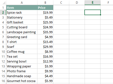
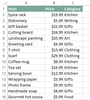
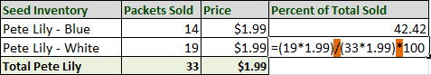
Basically, VLOOKUP lets you search for specific information in your spreadsheet. For example, if you have a list of products with prices, you could search for the price of a specific item.
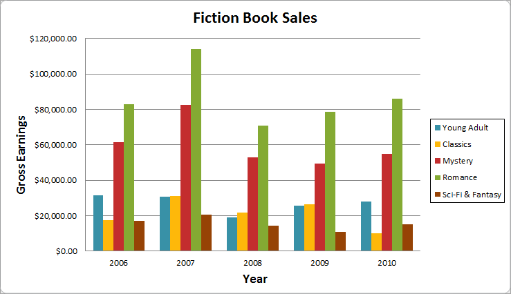
We’re going to use VLOOKUP to find the price of the Photo frame. You can probably already see that the price is $9.99, but that’s because this is a simple example. Once you learn how to use VLOOKUP, you’ll be able to use it with larger, more complex spreadsheets, and that’s when it will become truly useful.
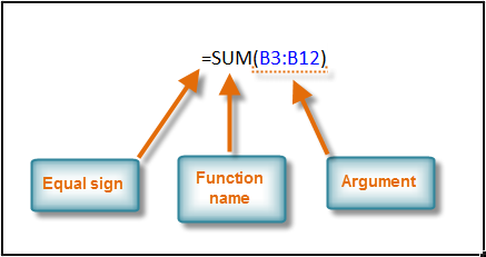
We’ll add our formula to cell E2, but you can add it to any blank cell. As with any formula, you’ll start with an equal sign (=). Then, type the formula name. Our arguments will need to be in parentheses, so type an open parenthesis. So far, it should look like this:
=VLOOKUP(
Adding the arguments
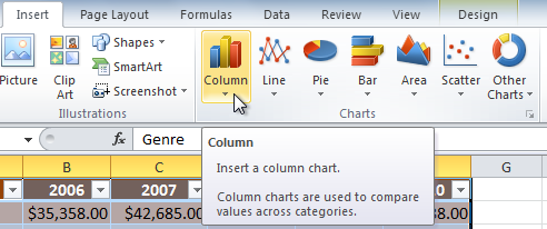
Now, we’ll add our arguments. The arguments will tell VLOOKUP what to search for and where to search.
The first argument is the name of the item you are searching for, which in this case is Photo frame. Since the argument is text, we’ll need to put it in double quotes:
=VLOOKUP(“Photo frame”
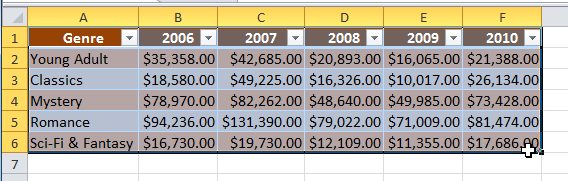
The second argument is the cell range that contains the data. In this example, our data is in A2:B16. As with any function, you’ll need to use a comma to separate each argument:
=VLOOKUP(“Photo frame”, A2:B16
Note: It’s important to know that VLOOKUP will always search the first column in this range. In this example, it will search column A for “Photo frame”. In some cases, you may need to move the columns around so that the first column contains the correct data.
The third argument is the column index number. It’s simpler than it sounds: The first column in the range is 1, the second column is 2, etc. In this case, we are trying to find the price of the item, and the prices are contained in the second column. That means our third argument will be 2:
=VLOOKUP(“Photo frame”, A2:B16, 2
The fourth argument tells VLOOKUP whether to look for approximate matches, and it can be either TRUE or FALSE. If it is TRUE, it will look for approximate matches. Generally, this is only useful if the first column has numerical values that have been sorted. Since we’re only looking for exact matches, the fourth argument should be FALSE. This is our last argument, so go ahead and close the parentheses:
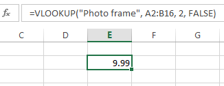
=VLOOKUP(“Photo frame”, A2:B16, 2, FALSE)
And that’s it! When you press enter, it should give you the answer, which is 9.99.
How it works
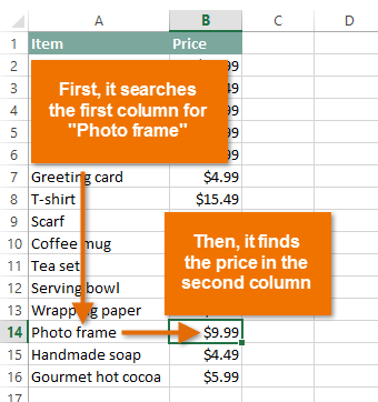
Let’s take a look at how this formula works. It first searches vertically down the first column (VLOOKUP is short for “vertical lookup”). When it finds “Photo frame”, it moves to the second column to find the price.
If we want to find the price of a different item, we can just change the first argument:
=VLOOKUP(“T-shirt”, A2:B16, 2, FALSE)
or:
=VLOOKUP(“Gift basket”, A2:B16, 2, FALSE)
Another example
OK, are you ready for a slightly more complicated example? Let’s say we have a third column that has the category for each item. This time, instead of finding the price, we’ll find the category.
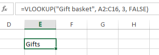
To find the category, we’ll need to change the second and third arguments in our formula. First, we’ll change the range to A2:C16 so that it includes the third column. Next, we’ll change the column index number to 3, since our categories are in the third column:
=VLOOKUP(“Gift basket”, A2:C16, 3, FALSE)
When you press Enter, you’ll see that the Gift basket is in the Gifts category.
Try it!
If you’d like more practice, see if you can find the following:
• The price of the coffee mug
• The category of the landscape painting
• The price of the serving bowl
• The category of the scarf
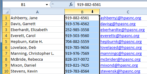
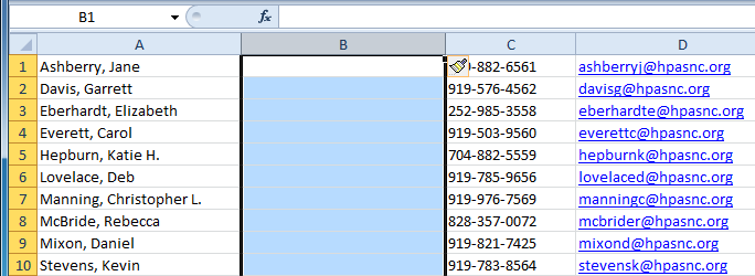
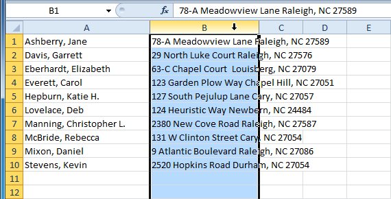
Now you know the basics of using VLOOKUP. Although advanced users sometimes use VLOOKUP in different ways, you can do a lot with the techniques that we’ve covered. For example, if you have a contact list, you could search for someone’s name to find their phone number. If your contact list has columns for the email address or company name, you could search for those by simply changing the second and third arguments, as we did in our example. The possibilities are endless!

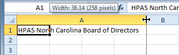
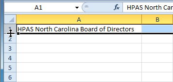
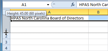
 becomes a double arrow
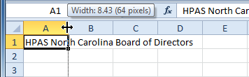
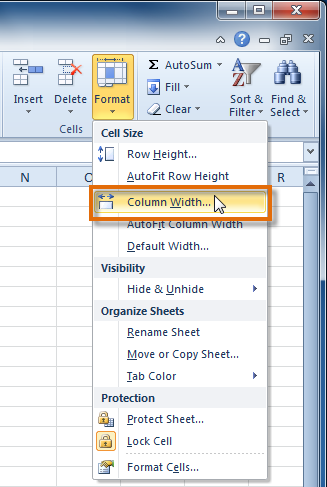
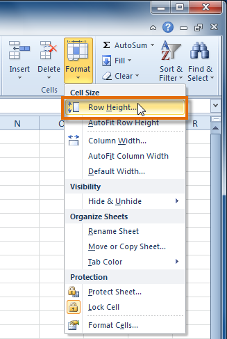
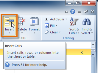
 by the inserted cells. This button allows you to choose how Excel formats them. By default, Excel formats inserted rows with the same formatting as the cells in the row above them. To access more options, hover your mouse over the Insert Options button and click on the drop-down arrow that appears.
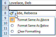

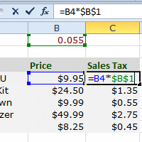
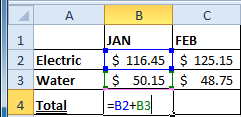

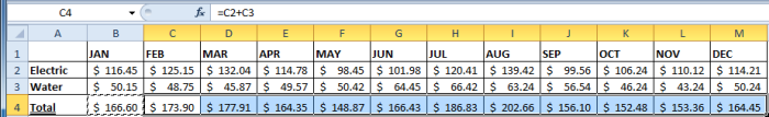
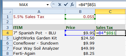
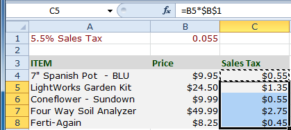
 Result in C4